Getting started with astir
Table of Contents:
0. Load necessary libraries
[39]:
# !pip install -e ../../..
import os
import sys
module_path = os.path.abspath(os.path.join('../../..'))
if module_path not in sys.path:
    sys.path.append(module_path)
[5]:
from astir.data import from_csv_yaml

import pandas as pd
import numpy as np
import matplotlib.pyplot as plt
import seaborn as sns

%load_ext autoreload
%autoreload 2
%matplotlib inline
1. Load data
We start by reading expression data in the form of a csv file and marker gene information in the form of a yaml file:
[1]:
expression_mat_path = "../../../tests/test-data/sce.csv"
# expression_mat_path = "data/sample_data.csv"
yaml_marker_path = "../../../tests/test-data/jackson-2020-markers.yml"
Note
Expression data should already be in a cleaned and normalized form. For IMC data, we perform this by an arcsinh transformation of the data with a cofactor so transformed_expression = archsinh(raw_expression / cofactor), where typically cofactor=5.
We can view both the expression data and marker data:
[2]:
!head -n 20 ../../../tests/test-data/jackson-2020-markers.yml
cell_states:
  RTK_signalling:
    - Her2
    - EGFR
  proliferation:
    - Ki-67
    - phospho Histone
  mTOR_signalling:
    - phospho mTOR
    - phospho S6
  apoptosis:
    - cleaved PARP
    - Cleaved Caspase3

cell_types:
  stromal:
    - Vimentin
    - Fibronectin
  B cells:
[6]:
pd.read_csv(expression_mat_path, index_col=0)[['EGFR','E-Cadherin', 'CD45', 'Cytokeratin 5']].head()
[6]:
| EGFR | E-Cadherin | CD45 | Cytokeratin 5 | |
|---|---|---|---|---|
| BaselTMA_SP41_186_X5Y4_3679 | 0.346787 | 0.938354 | 0.227730 | 0.095283 |
| BaselTMA_SP41_153_X7Y5_246 | 0.833752 | 1.364884 | 0.068526 | 0.124031 |
| BaselTMA_SP41_20_X12Y5_197 | 0.110006 | 0.177361 | 0.301222 | 0.052750 |
| BaselTMA_SP41_14_X1Y8_84 | 0.282666 | 1.122174 | 0.606941 | 0.093352 |
| BaselTMA_SP41_166_X15Y4_266 | 0.209066 | 0.402554 | 0.588273 | 0.064545 |
Then we can create an astir object using the from_csv_yaml function. For more data loading options, see the data loading tutorial.
[7]:
ast = from_csv_yaml(expression_mat_path, marker_yaml=yaml_marker_path)
print(ast)
Astir object, 6 cell types, 4 cell states, 100 cells
2. Fitting cell types
To fit cell types, simply call
[8]:
ast.fit_type(max_epochs=10, n_init=3, n_init_epochs=2)
training restart 1/3: 100%|██████████| 2/2 [ 4.51epochs/s, current loss: 745.5]
training restart 2/3: 100%|██████████| 2/2 [108.41epochs/s, current loss: 776.6]
training restart 3/3: 100%|██████████| 2/2 [40.70epochs/s, current loss: 774.7]
training restart (final): 100%|██████████| 10/10 [82.58epochs/s, current loss: 709.0]
/Users/jinelles.h/Documents/Camlab/astir-top-level/astir/astir/astir.py:178: UserWarning: Maximum epochs reached. More iteration may be needed to complete the training.
  warnings.warn(msg)
Note
Controlling inference There are many different options for controlling inference in the fit_type function, including max_epochs (maximum number of epochs to train), learning_rate (ADAM optimizer learning rate), batch_size (minibatch size), delta_loss (stops iteration once the change in loss falls below this value), n_inits (number of restarts using random initializations). For full details, see the function documentation.
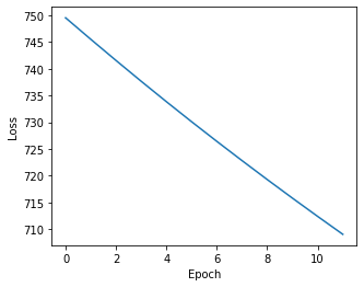
We should always plot the losses to assess convergence:
[9]:
plt.figure(figsize=(5,4))
plt.plot(np.arange(len(ast.get_type_losses())), ast.get_type_losses())
plt.ylabel("Loss")
plt.xlabel("Epoch")
[9]:
Text(0.5, 0, 'Epoch')
We can then get cell type assignment probabilities by calling
[10]:
assignments = ast.get_celltype_probabilities()
assignments
[10]:
| stromal | B cells | T cells | macrophage | epithelial(basal) | epithelial(luminal) | Other | |
|---|---|---|---|---|---|---|---|
| BaselTMA_SP41_186_X5Y4_3679 | 0.088444 | 0.084654 | 0.198811 | 0.105010 | 0.199379 | 0.119610 | 0.204091 |
| BaselTMA_SP41_153_X7Y5_246 | 0.110921 | 0.156938 | 0.193806 | 0.122539 | 0.200939 | 0.114491 | 0.100367 |
| BaselTMA_SP41_20_X12Y5_197 | 0.099029 | 0.107530 | 0.210399 | 0.135788 | 0.174190 | 0.126138 | 0.146926 |
| BaselTMA_SP41_14_X1Y8_84 | 0.117755 | 0.119934 | 0.221191 | 0.103741 | 0.150916 | 0.140125 | 0.146337 |
| BaselTMA_SP41_166_X15Y4_266 | 0.102338 | 0.106135 | 0.221755 | 0.135476 | 0.157753 | 0.125728 | 0.150815 |
| ... | ... | ... | ... | ... | ... | ... | ... |
| BaselTMA_SP41_114_X13Y4_1057 | 0.100268 | 0.128181 | 0.204113 | 0.140633 | 0.170518 | 0.111839 | 0.144448 |
| BaselTMA_SP41_141_X11Y2_2596 | 0.112603 | 0.143363 | 0.201669 | 0.148209 | 0.161044 | 0.116404 | 0.116708 |
| BaselTMA_SP41_100_X15Y5_170 | 0.111955 | 0.130958 | 0.203715 | 0.144000 | 0.163306 | 0.119814 | 0.126253 |
| BaselTMA_SP41_14_X1Y8_2604 | 0.076987 | 0.084889 | 0.218953 | 0.114034 | 0.200917 | 0.130515 | 0.173706 |
| BaselTMA_SP41_186_X5Y4_81 | 0.131032 | 0.128943 | 0.206584 | 0.123474 | 0.145218 | 0.125953 | 0.138796 |
100 rows × 7 columns
We can also visualize the assignment probabilities using a heatmap:
[11]:
sns.heatmap(assignments)
[11]:
<matplotlib.axes._subplots.AxesSubplot at 0x7f8041845410>
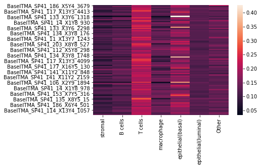
where each row corresponds to a cell, and each column to a cell type, with the entry being the probability of that cell belonging to a particular cell type.
To fetch an array corresponding to the most likely cell type assignments, call
[12]:
ast.get_celltypes()
[12]:
| cell_type | |
|---|---|
| BaselTMA_SP41_186_X5Y4_3679 | Unknown |
| BaselTMA_SP41_153_X7Y5_246 | Unknown |
| BaselTMA_SP41_20_X12Y5_197 | Unknown |
| BaselTMA_SP41_14_X1Y8_84 | Unknown |
| BaselTMA_SP41_166_X15Y4_266 | Unknown |
| ... | ... |
| BaselTMA_SP41_114_X13Y4_1057 | Unknown |
| BaselTMA_SP41_141_X11Y2_2596 | Unknown |
| BaselTMA_SP41_100_X15Y5_170 | Unknown |
| BaselTMA_SP41_14_X1Y8_2604 | Unknown |
| BaselTMA_SP41_186_X5Y4_81 | Unknown |
100 rows × 1 columns
Cell type diagnostics
It is important to run diagnostics to ensure that cell types express their markers at higher levels than other cell types. To do this, run the diagnostics_celltype() function, which will alert to any issues if a cell type doesn’t express its marker signficantly higher than an alternative cell type (for which that protein isn’t a marker):
[12]:
ast.diagnostics_celltype().head(n=10)
[12]:
| feature | should be expressed higher in | than | mean cell type 1 | mean cell type 2 | p-value | note |
|---|
Note
In this tutorial, we end up with many “Only 1 cell in a type: comparison not possible” notes - this is simply because the small dataset size results in only a single cell assigned to many types, making statistical testing infeasible.
Calling ast.diagnostics_celltype() returns a pd.DataFrame, where each column corresponds to a particular protein and two cell types, with a warning if the protein is not expressed at higher levels in the cell type for which it is a marker than the cell type for which it is not.
The diagnostics:
Iterates through every cell type and every marker for that cell type
Given a cell type c and marker g, find the set of cell types D that don’t have g as a marker
For each cell type d in D, perform a t-test between the expression of marker g in c vs d
If g is not expressed significantly higher (at significance alpha), output a diagnostic explaining this for further investigation.
If multiple issues are found, the markers and cell types may need refined.
3. Fitting cell state
Caution
Cell state fitting in Astir is currently experimental and not included in the initial paper.
Similarly as before, to fit cell state, call
[45]:
ast.fit_state(batch_size = 1024, learning_rate=1e-3, max_epochs=10)
/Users/jinelles.h/Documents/Camlab/astir-top-level/astir/astir/astir.py:222: UserWarning: Delta loss batch size is greater than the number of epochs
  warnings.warn("Delta loss batch size is greater than the number of epochs")
training restart 1/5: 100%|██████████| 5/5 [129.59epochs/s, current loss: 196.5]
training restart 2/5: 100%|██████████| 5/5 [117.63epochs/s, current loss: 231.9]
training restart 3/5: 100%|██████████| 5/5 [124.46epochs/s, current loss: 217.7]
training restart 4/5: 100%|██████████| 5/5 [88.48epochs/s, current loss: 275.4]
training restart 5/5: 100%|██████████| 5/5 [100.32epochs/s, current loss: 202.0]
training restart (final): 100%|██████████| 10/10 [92.36epochs/s, current loss: 170.3]
/Users/jinelles.h/Documents/Camlab/astir-top-level/astir/astir/astir.py:280: UserWarning: Maximum epochs reached. More iteration may be needed to complete the training.
  warnings.warn(msg)
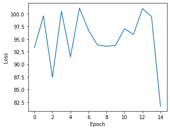
and similary plot the losses via
[14]:
plt.figure(figsize=(5,4))
plt.plot(np.arange(len(ast.get_state_losses())), ast.get_state_losses())
plt.ylabel("Loss")
plt.xlabel("Epoch")
[14]:
Text(0.5, 0, 'Epoch')
and cell state assignments can be inferred via
[15]:
states = ast.get_cellstates()
states
[15]:
| RTK_signalling | proliferation | mTOR_signalling | apoptosis | |
|---|---|---|---|---|
| BaselTMA_SP41_186_X5Y4_3679 | 0.568386 | 0.900861 | 0.656078 | 0.548110 |
| BaselTMA_SP41_153_X7Y5_246 | 0.421357 | 0.000000 | 0.524859 | 0.820946 |
| BaselTMA_SP41_20_X12Y5_197 | 0.944829 | 0.561159 | 0.979277 | 0.778787 |
| BaselTMA_SP41_14_X1Y8_84 | 0.858426 | 0.705787 | 0.938068 | 0.697319 |
| BaselTMA_SP41_166_X15Y4_266 | 0.933672 | 0.574031 | 0.980568 | 0.764967 |
| ... | ... | ... | ... | ... |
| BaselTMA_SP41_114_X13Y4_1057 | 0.881551 | 0.447002 | 0.899008 | 1.000000 |
| BaselTMA_SP41_141_X11Y2_2596 | 0.767853 | 0.684847 | 0.856773 | 0.722046 |
| BaselTMA_SP41_100_X15Y5_170 | 0.952977 | 0.548220 | 0.977899 | 0.786169 |
| BaselTMA_SP41_14_X1Y8_2604 | 0.836241 | 0.692617 | 0.908256 | 0.700867 |
| BaselTMA_SP41_186_X5Y4_81 | 0.691698 | 0.719179 | 0.705012 | 0.660071 |
100 rows × 4 columns
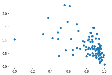
[16]:
plt.scatter(
    states['RTK_signalling'],
    ast.get_state_dataset().get_exprs_df()['Her2']
)
[16]:
<matplotlib.collections.PathCollection at 0x7f8041709d90>
Cell state diagnostics
It is important to run diagnostics on cell states model for the same reasons stated for the cell type model. Astir.diagnostics_cellstate() spots any non marker protein and pathway pairs whose expressions are higher than those of the marker proteins of the pathway.
[17]:
ast.diagnostics_cellstate().head(n=10)
[17]:
| pathway | protein A | correlation of protein A | protein B | correlation of protein B | note | |
|---|---|---|---|---|---|---|
| 0 | RTK_signalling | Her2 | -0.542371 | Ki-67 | -0.062491 | Her2 is marker for RTK_signalling but Ki-67 isn't |
| 1 | RTK_signalling | Her2 | -0.542371 | phospho S6 | -0.519752 | Her2 is marker for RTK_signalling but phospho ... |
| 2 | proliferation | Ki-67 | 0.241679 | Her2 | 0.344042 | Ki-67 is marker for proliferation but Her2 isn't |
| 3 | proliferation | Ki-67 | 0.241679 | phospho S6 | 0.411222 | Ki-67 is marker for proliferation but phospho ... |
| 4 | proliferation | Ki-67 | 0.241679 | phospho mTOR | 0.316836 | Ki-67 is marker for proliferation but phospho ... |
| 5 | mTOR_signalling | phospho mTOR | -0.776636 | Cleaved Caspase3 | -0.557334 | phospho mTOR is marker for mTOR_signalling but... |
| 6 | mTOR_signalling | phospho mTOR | -0.776636 | EGFR | -0.412919 | phospho mTOR is marker for mTOR_signalling but... |
| 7 | mTOR_signalling | phospho mTOR | -0.776636 | Her2 | -0.405998 | phospho mTOR is marker for mTOR_signalling but... |
| 8 | mTOR_signalling | phospho mTOR | -0.776636 | Ki-67 | -0.012072 | phospho mTOR is marker for mTOR_signalling but... |
| 9 | mTOR_signalling | phospho mTOR | -0.776636 | cleaved PARP | -0.557334 | phospho mTOR is marker for mTOR_signalling but... |
Calling ast.diagnostics_cellstate() returns a pd.DataFrame, where each column corresponds to a particular protein and two cell types, with a warning if the protein is not expressed at higher levels in the cell state for which it is a marker than the cell state for which it is not.
The diagnostics:
Get correlations between all cell states and proteins
For each cell state c, get the smallest correlation with marker g
For each cell state c and its non marker g, find any correlation that is bigger than those smallest correlation for c.
Any c and g pairs found in step 3 will be included in the output of
Astir.diagnostics_cellstate(), including an explanation.
If multiple issues are found, the markers and cell states may need refined.
4. Saving results
Both cell type and cell state information can easily be saved to disk via
[18]:
ast.type_to_csv("data/cell-types.csv")
ast.state_to_csv("data/cell-states.csv")
[19]:
!head -n 3 data/cell-types.csv
,cell_type
BaselTMA_SP41_186_X5Y4_3679,Unknown
BaselTMA_SP41_153_X7Y5_246,Unknown
[20]:
!head -n 3 data/cell-states.csv
,RTK_signalling,proliferation,mTOR_signalling,apoptosis
BaselTMA_SP41_186_X5Y4_3679,0.5683861877028941,0.9008611646823064,0.656078413193121,0.5481102160359178
BaselTMA_SP41_153_X7Y5_246,0.42135746208636826,0.0,0.5248592191573492,0.8209456743672588
where the first (unnamed) column always corresponds to the cell name/ID.
5. Accessing internal functions and data
Data stored in astir objects is in the form of an SCDataSet. These can be retrieved via
[21]:
celltype_data = ast.get_type_dataset()
celltype_data
[21]:
<astir.data.scdataset.SCDataset at 0x7f8041983290>
and similarly for cell state via ast.get_state_dataset().
These have several helper functions to retrieve relevant information to the dataset:
[22]:
celltype_data.get_cell_names()[0:4] # cell names
[22]:
['BaselTMA_SP41_186_X5Y4_3679',
 'BaselTMA_SP41_153_X7Y5_246',
 'BaselTMA_SP41_20_X12Y5_197',
 'BaselTMA_SP41_14_X1Y8_84']
[23]:
celltype_data.get_classes() # cell type names
[23]:
['stromal',
 'B cells',
 'T cells',
 'macrophage',
 'epithelial(basal)',
 'epithelial(luminal)']
[24]:
print(celltype_data.get_n_classes()) # number of cell types
print(celltype_data.get_n_features()) # number of features / proteins
6
14
[25]:
celltype_data.get_exprs() # Return a torch tensor corresponding to the expression data used
[25]:
tensor([[0.1026, 0.1004, 0.2277,  ..., 0.6097, 2.2151, 0.7714],
        [0.1081, 0.0176, 0.0685,  ..., 1.0622, 0.5026, 3.9632],
        [0.0498, 0.0943, 0.3012,  ..., 0.1601, 0.8102, 0.0481],
        ...,
        [0.0695, 0.0119, 0.0869,  ..., 0.4487, 0.7593, 1.4923],
        [0.0929, 0.1266, 0.2395,  ..., 0.4405, 2.2464, 0.4174],
        [0.0618, 0.1439, 0.2476,  ..., 0.7055, 3.1238, 0.2552]],
       dtype=torch.float64)
[26]:
celltype_data.get_exprs_df() # Return a pandas DataFrame corresponding to the expression data used
[26]:
| CD20 | CD3 | CD45 | CD68 | Cytokeratin 14 | Cytokeratin 19 | Cytokeratin 5 | Cytokeratin 7 | Cytokeratin 8/18 | E-Cadherin | Fibronectin | Her2 | Vimentin | pan Cytokeratin | |
|---|---|---|---|---|---|---|---|---|---|---|---|---|---|---|
| BaselTMA_SP41_186_X5Y4_3679 | 0.102576 | 0.100401 | 0.227730 | 2.227252 | 0.195163 | 0.190923 | 0.095283 | 0.057050 | 0.461040 | 0.938354 | 1.829905 | 0.609694 | 2.215089 | 0.771352 |
| BaselTMA_SP41_153_X7Y5_246 | 0.108137 | 0.017637 | 0.068526 | 0.208297 | 0.234853 | 0.685858 | 0.124031 | 0.485330 | 0.382767 | 1.364884 | 1.226994 | 1.062229 | 0.502627 | 3.963248 |
| BaselTMA_SP41_20_X12Y5_197 | 0.049809 | 0.094316 | 0.301222 | 0.581624 | 0.072666 | 0.115979 | 0.052750 | 0.035875 | 0.020290 | 0.177361 | 2.222520 | 0.160135 | 0.810243 | 0.048100 |
| BaselTMA_SP41_14_X1Y8_84 | 0.024256 | 0.140441 | 0.606941 | 0.490982 | 0.165863 | 0.652143 | 0.093352 | 0.351700 | 0.904383 | 1.122174 | 1.402750 | 1.133448 | 1.742495 | 1.917118 |
| BaselTMA_SP41_166_X15Y4_266 | 0.138571 | 0.111722 | 0.588273 | 1.039967 | 0.162696 | 0.086235 | 0.064545 | 0.009627 | 0.046967 | 0.402554 | 2.669947 | 0.558439 | 1.659587 | 0.687005 |
| ... | ... | ... | ... | ... | ... | ... | ... | ... | ... | ... | ... | ... | ... | ... |
| BaselTMA_SP41_114_X13Y4_1057 | 0.185995 | 0.049244 | 0.151869 | 0.296231 | 0.151970 | 0.175114 | 0.108374 | 0.021539 | 0.207346 | 2.120132 | 0.743909 | 1.460545 | 0.069651 | 1.666665 |
| BaselTMA_SP41_141_X11Y2_2596 | 0.100324 | 0.024006 | 0.025612 | 0.091424 | 0.049996 | 0.324138 | 0.083866 | 0.069627 | 0.614213 | 1.637392 | 0.860960 | 0.789372 | 0.000000 | 2.584532 |
| BaselTMA_SP41_100_X15Y5_170 | 0.069503 | 0.011859 | 0.086852 | 0.538247 | 0.037131 | 0.321179 | 0.096496 | 0.000000 | 0.696445 | 0.861641 | 1.724828 | 0.448688 | 0.759268 | 1.492342 |
| BaselTMA_SP41_14_X1Y8_2604 | 0.092944 | 0.126645 | 0.239459 | 1.967150 | 0.171216 | 0.132563 | 0.055748 | 0.082334 | 0.128377 | 0.532135 | 1.899111 | 0.440527 | 2.246434 | 0.417445 |
| BaselTMA_SP41_186_X5Y4_81 | 0.061784 | 0.143930 | 0.247627 | 0.316248 | 0.232111 | 0.145036 | 0.080324 | 0.000000 | 0.208533 | 0.899182 | 2.475906 | 0.705456 | 3.123784 | 0.255158 |
100 rows × 14 columns
[27]:
ast.normalize()
[28]:
ast.get_type_dataset().get_exprs_df()
[28]:
| CD20 | CD3 | CD45 | CD68 | Cytokeratin 14 | Cytokeratin 19 | Cytokeratin 5 | Cytokeratin 7 | Cytokeratin 8/18 | E-Cadherin | Fibronectin | Her2 | Vimentin | pan Cytokeratin | |
|---|---|---|---|---|---|---|---|---|---|---|---|---|---|---|
| BaselTMA_SP41_186_X5Y4_3679 | 0.020514 | 0.020079 | 0.045530 | 0.384408 | 0.039023 | 0.038175 | 0.019055 | 0.011410 | 0.092078 | 0.186586 | 0.358267 | 0.121639 | 0.429674 | 0.153665 |
| BaselTMA_SP41_153_X7Y5_246 | 0.021626 | 0.003527 | 0.013705 | 0.041647 | 0.046953 | 0.136745 | 0.024804 | 0.096914 | 0.076479 | 0.269695 | 0.243000 | 0.210879 | 0.100357 | 0.726918 |
| BaselTMA_SP41_20_X12Y5_197 | 0.009962 | 0.018862 | 0.060208 | 0.116064 | 0.014533 | 0.023194 | 0.010550 | 0.007175 | 0.004058 | 0.035465 | 0.431033 | 0.032021 | 0.161348 | 0.009620 |
| BaselTMA_SP41_14_X1Y8_84 | 0.004851 | 0.028085 | 0.121092 | 0.098039 | 0.033167 | 0.130062 | 0.018669 | 0.070282 | 0.179905 | 0.222592 | 0.276994 | 0.224792 | 0.341804 | 0.374601 |
| BaselTMA_SP41_166_X15Y4_266 | 0.027711 | 0.022343 | 0.117385 | 0.206522 | 0.032533 | 0.017246 | 0.012909 | 0.001925 | 0.009393 | 0.080424 | 0.511404 | 0.111457 | 0.326107 | 0.136972 |
| ... | ... | ... | ... | ... | ... | ... | ... | ... | ... | ... | ... | ... | ... | ... |
| BaselTMA_SP41_114_X13Y4_1057 | 0.037190 | 0.009849 | 0.030369 | 0.059212 | 0.030389 | 0.035016 | 0.021673 | 0.004308 | 0.041457 | 0.412250 | 0.148238 | 0.288107 | 0.013930 | 0.327450 |
| BaselTMA_SP41_141_X11Y2_2596 | 0.020063 | 0.004801 | 0.005122 | 0.018284 | 0.009999 | 0.064782 | 0.016772 | 0.013925 | 0.122536 | 0.321891 | 0.171352 | 0.157226 | 0.000000 | 0.496282 |
| BaselTMA_SP41_100_X15Y5_170 | 0.013900 | 0.002372 | 0.017370 | 0.107443 | 0.007426 | 0.064192 | 0.019298 | 0.000000 | 0.138843 | 0.171486 | 0.338466 | 0.089618 | 0.151276 | 0.294206 |
| BaselTMA_SP41_14_X1Y8_2604 | 0.018588 | 0.025326 | 0.047873 | 0.383928 | 0.034236 | 0.026509 | 0.011149 | 0.016466 | 0.025673 | 0.106227 | 0.371236 | 0.087992 | 0.435399 | 0.083392 |
| BaselTMA_SP41_186_X5Y4_81 | 0.012356 | 0.028782 | 0.049505 | 0.063207 | 0.046406 | 0.029003 | 0.016064 | 0.000000 | 0.041695 | 0.178881 | 0.476898 | 0.140627 | 0.589937 | 0.051009 |
100 rows × 14 columns
6. Saving models
After fixing the models, we can save the cell type/state assignment, the losses, the parameters (e.g. mu, rho, log_sigma, etc) and the run informations (e.g. batch_size, learning_rate, delta_loss, etc) to an hdf5 file.
[29]:
ast.save_models("data/astir_summary.hdf5")
The hierarchy of the hdf5 file would be:
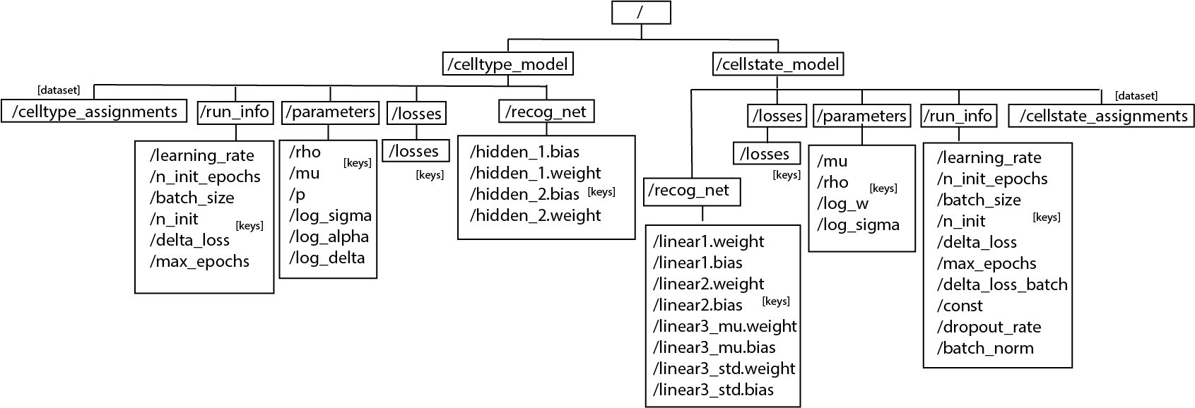
Only the model that is trained will be saved (CellTypeModel or CellStateModel or both). If the functioned is called before any model is trained, exception will be raised. Data saved in the file is either int or np.array.
7. Plot clustermap of expression data
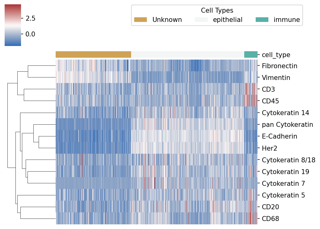
After fixing the cell type model, we can also plot a heatmap of protein expression of cells clustered by type. The heatmap will be saved at the location plot_name, which is default to "./celltype_protein_cluster.png"
[30]:
ast.type_clustermap(plot_name="./img/celltype_protein_cluster.png", threshold = 0.7, figsize=(7, 5))
Note: threshold is the probability threshold above which a cell is assigned to a cell type, default to 0.7.
8. Hierarchical model specification
In the marker yaml file, the user can also add a section called hierarchy, which specifies the hierarchical structure of cell types. Here’s an example:
hierarchy:
    epithelial_cells:
        - epithelial(luminal)
        - epithelial(basal)
    immune cells:
        non-lymphocytes:
            - macrophage
        lymphocytes:
            - T cells
            - B cells
Some notes: 1. The section would be accessed by key hierarchy. 2. In the section, the higher-levelled cell type names should be the keys. 3. The values in the section should also exist as the cell type names in the cell_types section. (e.g. if we have "B cells" in marker["hierarchy"]["immune"], we should also be able to get marker["cell_types"]["B cells"]) 4. In terms of depth in the example: - depth=1: assign to epithelial_cells or immune_cells - depth=2: assign to
epithelial(luminal), epithelial(basal), non-lymphocyte and lymphocyte - depth=3: assign to epithelial(luminal), epithelial(basal), macrophage, T cells and B cells
This section could be used to summarize the cell types assignment at a higher hierarchical level. (e.g. a cell is predicted as “immune” instead of “B cells” or “T cells”)
[31]:
hierarchy_probs = ast.assign_celltype_hierarchy(depth = 1)
hierarchy_probs.head()
[31]:
| epithelial_cells | immune cells | |
|---|---|---|
| BaselTMA_SP41_186_X5Y4_3679 | 0.318990 | 0.388475 |
| BaselTMA_SP41_153_X7Y5_246 | 0.315430 | 0.473283 |
| BaselTMA_SP41_20_X12Y5_197 | 0.300328 | 0.453717 |
| BaselTMA_SP41_14_X1Y8_84 | 0.291041 | 0.444866 |
| BaselTMA_SP41_166_X15Y4_266 | 0.283482 | 0.463366 |
[32]:
hierarchy_probs = ast.assign_celltype_hierarchy(depth = 2)
hierarchy_probs.head()
[32]:
| epithelial(luminal) | epithelial(basal) | non-lymphocytes | lymphocytes | |
|---|---|---|---|---|
| BaselTMA_SP41_186_X5Y4_3679 | 0.119610 | 0.199379 | 0.105010 | 0.283465 |
| BaselTMA_SP41_153_X7Y5_246 | 0.114491 | 0.200939 | 0.122539 | 0.350744 |
| BaselTMA_SP41_20_X12Y5_197 | 0.126138 | 0.174190 | 0.135788 | 0.317929 |
| BaselTMA_SP41_14_X1Y8_84 | 0.140125 | 0.150916 | 0.103741 | 0.341125 |
| BaselTMA_SP41_166_X15Y4_266 | 0.125728 | 0.157753 | 0.135476 | 0.327890 |
[33]:
hierarchy_probs = ast.assign_celltype_hierarchy(depth = 3)
hierarchy_probs.head()
[33]:
| epithelial(luminal) | epithelial(basal) | macrophage | T cells | B cells | |
|---|---|---|---|---|---|
| BaselTMA_SP41_186_X5Y4_3679 | 0.119610 | 0.199379 | 0.105010 | 0.198811 | 0.084654 |
| BaselTMA_SP41_153_X7Y5_246 | 0.114491 | 0.200939 | 0.122539 | 0.193806 | 0.156938 |
| BaselTMA_SP41_20_X12Y5_197 | 0.126138 | 0.174190 | 0.135788 | 0.210399 | 0.107530 |
| BaselTMA_SP41_14_X1Y8_84 | 0.140125 | 0.150916 | 0.103741 | 0.221191 | 0.119934 |
| BaselTMA_SP41_166_X15Y4_266 | 0.125728 | 0.157753 | 0.135476 | 0.221755 | 0.106135 |
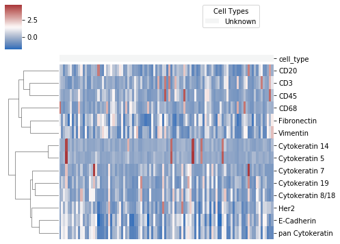
To make it more clear, here’s a heatmap for the cell assignment in a higher hierarchy:
The way it is calculated is simply summing up the probabilities of the cell type assignments under the same hierarchy.
9. Using astir as command line tool
astir could also be used as a command line tool with csv input. Here are some example.
To fit cell types on the sample csv file and marker with a design matrix, setting n_init to 3 and batch_size to 128:
[44]:
!astir type ../../../tests/test-data/test_data.csv ../../../tests/test-data/jackson-2020-markers.yml data/test_data_type_assignments.csv --design ../../../tests/test-data/design.csv --n_init 3 --batch_size 128
training restart 1/3: 100%|██████████| 5/5 [164.98epochs/s, current loss: -25.6]
training restart 2/3: 100%|██████████| 5/5 [181.48epochs/s, current loss: -33.4]
training restart 3/3: 100%|██████████| 5/5 [177.48epochs/s, current loss: -12.5]
training restart (final): 100%|███| 50/50 [198.48epochs/s, current loss: -591.9]
/Users/jinelles.h/Documents/Camlab/astir-top-level/astir/astir/astir.py:178: UserWarning: Maximum epochs reached. More iteration may be needed to complete the training.
  warnings.warn(msg)
To fit cell states on the sample csv file and marker, setting learning rate to 5e-4, dropout_rate to 0.2 and batch_norm to True:
[43]:
!astir state ../../../tests/test-data/test_data.csv ../../../tests/test-data/jackson-2020-markers.yml data/test_data_type_assignments.csv --design ../../../tests/test-data/design.csv --learning_rate 5e-4 --dropout_rate 0.2 --batch_norm True
training restart 1/3: 100%|████████| 5/5 [142.02epochs/s, current loss: 32237.3]
training restart 2/3: 100%|██████████| 5/5 [226.10epochs/s, current loss: 963.2]
training restart 3/3: 100%|███████| 5/5 [230.45epochs/s, current loss: 147046.4]
training restart (final):   0%|          | 0/50 [?epochs/s, current loss: 883.6]
Moreover, astir could also be used as a converter which converts rds file with SingleCellExperiment to csv file. see more details
Run astir -h, astir type -h, astir state -h and astir convert -h in the command line for more details.
[33]: